RD-A7
A four-rotor inspection platform that flies repeatable survey lines over fixed assets and returns georeferenced visual and radiometric data. Built around one idea: a flight is only useful if the next one can be compared against it.
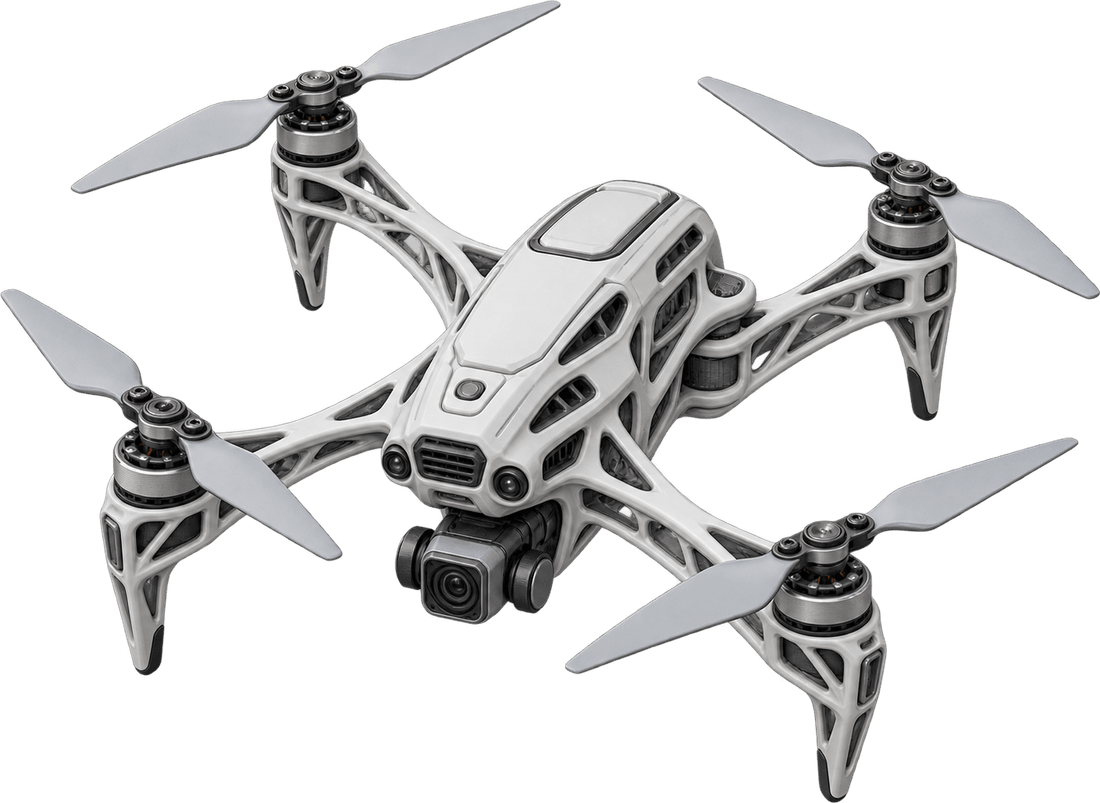
Programme visualization of the lattice-structure airframe. The structural qualification gates for this geometry are documented below.
The problem
Most asset inspection produces photographs. Photographs cannot be subtracted from each other.
A corroding weld, a delaminating blade, a bus-bar running warm — each is a change over time rather than a state at a moment. Detecting change requires that two surveys flown months apart put the same pixel on the same feature, which is a positioning problem long before it is an imaging or a machine learning problem. Nearly every design decision below follows from taking that requirement seriously.
Flight physics
Hover power is not a design choice — momentum theory fixes it from mass and disc area. The rotor accelerates a column of air downward, and the power required is set by how much air it can work on.
Phover = (mg)3/2 / [ FM · √(2 ρA) ]
The exponent is what matters. Power grows with mass3/2, so the last kilogram of payload costs more endurance than the first, and no amount of motor efficiency changes that relationship. Disc area is the only term that pushes back, which is why the airframe is larger than the payload alone would suggest.
t = Epack · DoD / ( Phover + Pavionics )
Holding station in wind is a smaller thrust problem than people expect. The aircraft tilts until the horizontal component of thrust balances drag, and at 12 m/s that angle is on the order of ten degrees — which raises required thrust by under two percent.
tan θ = D / W , D = ½ ρ v2 CdA , T = W / cos θ
Structural qualification
The lattice airframe is a load path, not a visual treatment.
Open truss and topology-optimized structures can remove material from regions carrying little load, but a hollow shape is not automatically an efficient or safe one. The geometry must be generated from the aircraft's actual load cases, protected around interfaces that cannot move, constrained by the chosen manufacturing process, and then correlated against physical test articles.
For RD-A7, the structural model has to include maximum rotor thrust, combined manoeuvre and gust loading, asymmetric thrust, landing and handling loads, payload and parachute attachment reactions, and the inertia of the battery and sensor package. Motor mounts, arm roots, fuselage junctions and landing-leg transitions are retained as non-design regions because their interfaces are set by hardware, not by the optimizer.
| Question | Verification method | Required evidence |
|---|---|---|
| Does it carry the defined flight and ground loads? | Linear static FEA followed by nonlinear analysis where joints, large deflection or contact make linear assumptions invalid. | Stress, displacement, joint load and margin results for every governing load case. |
| Will an arm twist enough to corrupt control or imaging? | Torsional-stiffness analysis and physical twist testing at the motor interface. | Measured stiffness correlated with the model and held inside flight-control and sensor-pointing limits. |
| Can rotor excitation reach a structural mode? | Modal FEA followed by a ground-vibration or instrumented impact test on the assembled airframe. | Natural frequencies and mode shapes with defined separation from rotor, blade-pass and control-loop excitation. |
| Can slender lattice members buckle? | Eigenvalue screening followed by nonlinear buckling analysis for the compression-critical cases. | Positive buckling margin after geometric imperfection and manufacturing tolerance are included. |
| Will repeated flights initiate fatigue damage? | Load-spectrum definition, strain measurement and representative fatigue or accelerated cycle testing. | Life estimate and inspection intervals for arm roots, lattice nodes, mounts and landing structure. |
| Does the manufactured material behave like the model? | Process-specific coupons and witness specimens tested in the relevant build orientations and environmental conditions. | Allowables for stiffness, strength and variability—not handbook values for unprocessed bulk material. |
The qualification gate
Analysis releases a test article; it does not release a flight vehicle. The assembled structure must pass proof loading at the requirement-derived test level, ground-vibration testing, the defined vibration spectrum, repeated landing and handling cycles, and post-test inspection. Strain and displacement measured during those tests are compared with the finite-element model. A material change, altered print orientation, revised arm geometry or moved payload invalidates the affected correlation and reopens the relevant tests.
The airframe shown on this page is therefore a programme design configuration, not evidence of structural qualification. It becomes flight-qualified only when the analytical margins and physical results agree within the acceptance criteria defined for the platform.
Positioning
The GNSS receiver is integrated rather than a bolt-on: multi-band and multi-constellation, tracking GPS L1/L2/L5, Galileo E1/E5, GLONASS and BeiDou simultaneously. Multi-band matters more than constellation count, because a second frequency lets the receiver solve the ionospheric delay directly instead of modelling it, and it makes carrier-phase ambiguity resolution converge in seconds rather than minutes.
Standalone GNSS gives metre-level position, which is useless for comparing two surveys. RTK resolves the carrier-phase ambiguity against a reference and brings that to roughly two centimetres. Corrections arrive over the network by NTRIP, so no base station has to be surveyed in and set up on site — which removes the single most common reason a survey slips a day.
Where the network is unreachable, the receiver logs raw observables and the flight is post-processed against a reference station afterwards. PPK gives the same centimetre geometry with the corrections applied later, so a lost link degrades the schedule rather than the survey.
Heading without a magnetometer
This is the part that matters near steel. A magnetometer alongside a transformer, a tank wall or a substation gantry reads the structure, not the earth — and heading error feeds straight into georeferencing error. Two GNSS antennas on a fixed baseline solve heading from the carrier-phase difference between them instead, with no magnetic dependence at all.
σψ ≈ arctan( σrel / L ) ≈ arctan( 3 mm / 0.55 m ) ≈ 0.3°
Inside tank farms and under structures, GNSS fails outright — multipath corrupts the fix long before the signal disappears, which is the dangerous failure because the receiver still reports a position. The platform falls back to visual-inertial odometry fused with the IMU, tracks which source it is trusting, and publishes an honest covariance rather than an optimistic one. A planner that believes an overconfident pose is a planner that flies into a handrail.
Holding the standoff
Ground sample distance is proportional to standoff, so altitude error is resolution error. Holding GSD within five percent means holding height above the surface within five percent — about fifteen centimetres at a three-metre standoff.
ΔGSD / GSD = ΔH / H
The flight plan is therefore terrain-following against a prior surface model, with the radar altimeter closing the loop on what is actually beneath the aircraft. Every frame in the survey lands at the same resolution, which is the precondition for comparing one survey against the next.
What it can see
Detection is set by optics and standoff, not by the model doing the looking. Ground sample distance falls directly out of sensor geometry, and a feature must span at least three pixels before it is separable from sensor noise and demosaicing artefacts.
GSD = H · p / f → dmin ≈ 3 · GSD
This makes the survey plan a resolution decision before it is a coverage decision. Doubling altitude to halve the flight time also doubles the smallest detectable defect, and that trade should be made explicitly against the defect size the inspection is actually looking for — not discovered afterwards when nothing was found.
A mechanical shutter is not a refinement here. A rolling shutter exposes the frame line by line, so at 15 m/s the top and bottom of an image are taken from measurably different positions, shearing the geometry. That distortion is larger than the defects being looked for, and it corrupts photogrammetry downstream as well.
The thermal channel is radiometric rather than a false-colour picture: every pixel carries an absolute temperature, so a hotspot can be compared against a threshold and against last quarter's flight. NETD below 50 mK sets the smallest temperature difference that is distinguishable from sensor noise, which for a bolted electrical connection is the difference between catching degradation and catching a failure.
Avoiding things
Obstacle sensing is omnidirectional stereo vision paired with 60 GHz mmWave radar, and the pairing is deliberate rather than redundant. Stereo vision has far better angular resolution and fails in exactly the conditions industrial sites produce: dust, steam, fog, rain, low light, and the blank untextured surfaces of tank walls where correspondence matching has nothing to match.
Radar is coarse but nearly indifferent to all of it, and it measures range directly rather than inferring it. Neither sensor covers the other's failure mode by being better; they cover it by failing for unrelated reasons, which is the only kind of redundancy worth paying for.
When something fails
Inertial sensing is triple-redundant with median voting. The reason it is three and not two is a detection-versus-isolation argument: two sensors that disagree tell you one has failed but not which, leaving nothing safe to do except abort. Three let the odd one out be identified and excluded, and the flight continues on the remaining pair.
Barometers are dual with cross-check, the geofence is enforced below the flight-planning layer so a bad plan cannot cross it, and link loss triggers a return along the flown path rather than a straight line home — because the straight line is the one that has not been checked for obstacles.
Last-resort recovery is a ballistic parachute. Canopy area is solved backwards from the descent rate rather than chosen, and the descent rate is set by the impact energy considered survivable.
vdescent = √( 2mg / ρ Cd S ) → Eimpact = ½ m v2
Deciding onboard
Inference runs on the aircraft, and the reason is arithmetic rather than preference. A single 20 MP frame at 12 bits is roughly 30 MB. The command link sustains about 20 Mbit/s, so transmitting one frame takes around twelve seconds — against a survey cadence of one to two frames per second.
ttx = Sframe · 8 / Rlink ≈ 240 Mbit / 20 Mbit·s−1 ≈ 12 s
So the link carries conclusions rather than data: detections, confidence, and georeferenced crops around anything flagged. Full-resolution imagery is written to onboard storage and recovered after landing. The operator sees findings in flight; the archive survives for the next comparison.
Identity and data
The aircraft holds a private key generated inside a hardware secure element and never exported, so it can prove which airframe it is without that credential existing anywhere it could be copied. Firmware is signature-verified with rollback protection, and the anti-rollback counter only advances after the new image has booted and reported itself healthy — otherwise a failed update leaves a device that can run neither version.
Survey data is encrypted at rest. It routinely contains the physical layout and condition of critical infrastructure, which is sensitive on its own terms regardless of who owns the asset. Broadcast Remote ID and ADS-B In are carried because they are regulatory requirements in the jurisdictions this class of aircraft operates in, not as features.
Specification
| Maximum take-off mass | 4.2 kg |
|---|---|
| Usable payload | 1.2 kg |
| Diagonal span | 900 mm |
| Rotor disc area | 0.55 m² (4 × Ø 420 mm) |
| Pack energy | 266 Wh (6S, 12 Ah) |
| Hover power at MTOW (electrical) | ≈ 350 W |
| Endurance at MTOW | 36 min |
| Cruise speed | 15 m/s |
| Sustained wind | 12 m/s |
| GNSS receiver | Integrated multi-band, multi-constellation |
| Constellations | GPS L1/L2/L5 · Galileo E1/E5 · GLONASS · BeiDou |
| RTK corrections | Network NTRIP over LTE — no site base station |
| Positioning (RTK fixed) | ± 2 cm horizontal, ± 3 cm vertical |
| Fallback positioning | PPK from logged raw observables |
| Heading | Dual-antenna GNSS, 0.55 m baseline, ± 0.3° |
| GNSS-denied navigation | Visual-inertial odometry, IMU-fused |
| Altitude hold | Radar altimeter, ± 5 cm above surface |
| Obstacle sensing | Omnidirectional stereo + 60 GHz mmWave radar |
| Inertial redundancy | Triple IMU, median voting · dual barometer |
| Primary sensor | 20 MP 4/3 CMOS, mechanical shutter |
| Radiometric thermal | 640 × 512, NETD < 50 mK, ± 2 °C |
| Optional payloads | LiDAR · multispectral · gas sensing |
| Onboard compute | Edge inference, detection in flight |
| Storage | AES-256 encrypted at rest |
| Device identity | Hardware secure element, signed firmware |
| Command link | AES-256, 8 km line of sight |
| Recovery | Ballistic parachute, Ø 1.2 m canopy |
| Structural validation | FEA-to-test correlation and flight qualification required |
| Compliance | Broadcast Remote ID · ADS-B In |
| Environmental | IP54, −20 °C to +50 °C |
These figures are coupled. Mass, disc area and pack energy determine hover power and therefore endurance; canopy area is solved from the descent target; heading accuracy follows from the antenna baseline. Changing one moves the others.
Inspecting something that has to be measured, not photographed?
The interesting constraint is usually the smallest defect that matters and how often it has to be checked. Those two numbers set the platform.